A couple of years ago I was interested in the efficiency of R when it comes to time processing and management of memory and I read a few blog posts about this topic, particularly pointing at the fact that R hasn't been designed to be a very efficient language, especially when it comes to big data processing, and this could be its doom at some point in the future. By that time I also read a great article or blog post regarding the complexity of using the tidyverse family of packages in R, especially with the task of teaching R to beginners. The text made excellent points discussing how the syntax of tidyverse packages is so different from the base R functions that it might confuse the people trying to learn R from scratch. Thus, the narration continued towards the use of the packages data.table instead, which maintains a syntax closer to that of base R. And from there, the author also took the opportunity to discuss efficiency of both packages. I apologize for the lack of sources but I could not find the link to the post(s) I'm referring to, if any of you knows the post I'm talking about please, share the link with me, I'd be greatly thankful.
Regardless of that line of thinking, I believe that we can all feel lucky to have packages such as tidyverse and data.table which make time processing of big data easier, among other advantages. And these are only the beginning to the list of packages. Although I was interested in the topic myself, I never run some "formal tests" to compare the efficiency of this or other packages (although I was comparing a few languages including Julia, Common Lisp and of course, Python, similarly to niklas-heer in his speed-comparison repo, to whom I also thank for my head image). Nevertheless, in the last couple of weeks I had to do such tests due to the nature of my current job.
I recently joined a project where the team has been developing a mapper and wrapper of data using R, where the input data can vary from 2 rows to a few millions. The whole process runs through couple of servers to import the data into R, process it accordingly and send it out to a data base from where is served into some other software. The whole process per-se is quite complex and due to the use of servers and Internet connections it can become quite slow. Thus, it is critical that the time processing in R is efficient.
As mentioned before, a team has been working on this project for a while and they were using the tidyverse family of packages a lot. Myself I prefer to stick to base R functions when it comes to development. I think it makes the work neat, simple and easier, keeps the dependencies to the minimum and, since I know R for more than 10 years, it's easier for me to write code in base R. And please, don't misunderstand me, I like the tidyverse functions but I rather use them when it comes to data analysis: it is great to clean data, prepare it to fit models, explore it, and of course, to make visualizations with the wonderful ggplot preceded by the %>% sequence to provide exactly what is needed. But for me, developing a software in base R is just more straight forward.
However, as I said, efficiency is critical in this project and thus, I've been tasked to test it in a few functions already. The most recent was a function to import JSON files line by line using dplyr functions which I could reduce by half the time using data.table functions, but that's a topic for another time. One of the first tasks I was given as a new member was to map a process, very similar to another one but with different input parameters. I could had simply copied the code from the previous mapping process into my own script and just change the parameters, since the mapping logic is exactly the same. However, I decided to create my own code using base R, trusting that is more straight forward and efficient, and at the same time taking the opportunity to show up my skills to my new team. Therefore, I ended up comparing the efficiency of the functions using Monte Carlo simulations and thus, creating the present post. I hope it can be useful for some of you.
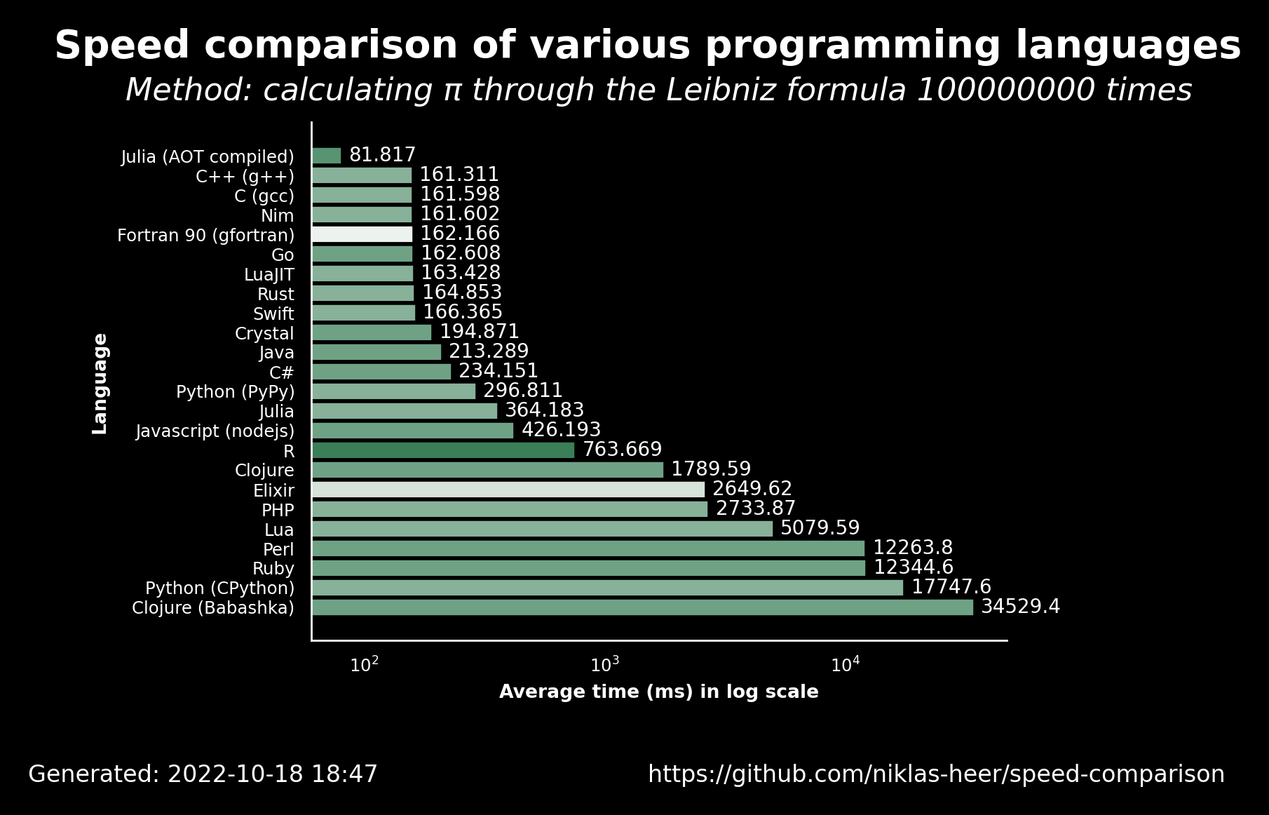
| Image 1. Credits - https://github.com/niklas-heer/speed-comparison |
The task
The general idea is to map a RESPONSE based on the contents of one column, in this case CODE1: all values get the response "BATCH", but only when CODE1 is empty, they also get the response "GETTING". Rows with value "BATCH" get renamed the columns NAME, DAY and TIME into TEAM, RESPONSETD and RESPONSESTT respectively, while rows with response "GETTING" only get one more column: NAME into newly named column TEAM.
(test.df <- data.frame(NAME = as.character(c(1:10)),
                      DAY = format(Sys.time(), "%d-%m-%y"),
                      TIME = format(Sys.time(), "%T"),
                      CODE1 = c("Code", NA)))
>    NAME      DAY     TIME CODE1
> 1     1 20-10-22 18:37:23  Code
> 2     2 20-10-22 18:37:23  <NA>
> 3     3 20-10-22 18:37:23  Code
> 4     4 20-10-22 18:37:23  <NA>
> 5     5 20-10-22 18:37:23  Code
> 6     6 20-10-22 18:37:23  <NA>
> 7     7 20-10-22 18:37:23  Code
> 8     8 20-10-22 18:37:23  <NA>
> 9     9 20-10-22 18:37:23  Code
> 10   10 20-10-22 18:37:23  <NA>
The whole general idea is to create a new table with response values, which follows and is followed by a series of adjustments to the data. For the post I have created a test data frame with simple values, in case somebody would like to reproduce the code execution.
rename_nCols <- function(samples, cols_to_rename, rename = FALSE, ignore_missing = TRUE){
  for(i in 1:length(cols_to_rename)){
    old_name <- cols_to_rename[[i]][1] ## Old in position 1 of vector
    SYS_name <- cols_to_rename[[i]][2] ## New in position 2 of vector
    ## WHEN NOT PRESENT
    if(!old_name %in% names(samples)) {
      warning(paste("Column", old_name, "not found."))
      if(!ignore_missing){
        samples[,SYS_name] <- as.character(NA)
      }
    }
    ## RENAMING
    else if(rename){
      names(samples)[names(samples) == old_name] <- SYS_name
    }
    ## ADDING
    else {
      samples[,SYS_name] <- samples[,old_name]
    }
  }
  return(samples)
}

create_cols_base <- function(samples){
  require(dplyr)
  ## First BATCH
  assay <- cbind(samples, RESPONSE = "BATCH")
  cols_to_rename <- list(c('NAME', 'TEAM'),
                         c('DAY', 'RESPONSETD'),
                         c('TIME', 'RESPONSESTT'))
  assay <- rename_nCols(assay, cols_to_rename)
  ## then GETTING
  if("CODE1" %in% names(samples)){
    if(nrow(samples[is.na(samples$CODE1),]) != 0){
      receiving <- cbind(samples[is.na(samples$CODE1),], RESPONSE = "GETTING")
    }
    else receiving <- samples[is.na(samples$CODE1),]
  }
  else{
    receiving <- cbind(samples, RESPONSE = "GETTING")
  }
  receiving <- rename_nCols(receiving, list(c('NAME', 'TEAM')))
  responses <- full_join(assay, receiving)
  return(responses)
}
My strategy using base R (function create_cols_base()) was to create two data frames, one per each response, and then join them using full_join() from dplyr. I want to stress that the idea was never to use only base R but rather to follow my own logic and my knowledge of R and then compare it with that of my colleagues. To support my create_cols_base() I created a function rename_nCols which is a great asset to the project since we are constantly renaming columns or creating new ones based on old ones.
create_cols_tidy <- function(samples, responsesToCreate = c("BATCH", "GETTING")){
    require(dplyr)
    require(tidyr)
  responses <- samples %>%
    mutate(
      RESPONSE =
        case_when(
          is.na(get0('CODE1', ifnotfound = as.character(NA))) |
          get0('CODE1', ifnotfound = as.character(NA)) == "" ~
              list(Reduce(intersect,list(responsesToCreate,c("BATCH", "GETTING")))),
          TRUE ~ list(Reduce(intersect,list(responsesToCreate,c("BATCH"))))
        )
    ) %>%
      unnest(cols = c(RESPONSE))%>%
      subset(!is.na(RESPONSE)) %>%
      mutate(TEAM = get0('NAME', ifnotfound = as.character(NA)),
             RESPONSESTD = case_when(
             (RESPONSE == "BATCH") ~ get0('DAY', ifnotfound = as.character(NA)),
             TRUE ~ as.character(NA)),
             RESPONSESTTM = case_when(
             (RESPONSE == "BATCH") ~ get0('TIME', ifnotfound = as.character(NA)),
             TRUE ~ as.character(NA)))
    return(responses)
}
As you can see in the code chunk above, my colleagues decided to use a completely different approach, with the function case_when() as the protagonist. An excellent call in my opinion, but one I'm not so familiar with in R. They also made use of the strength of mutate() to reduce generation of excessive data frames, as it was my case.
The test
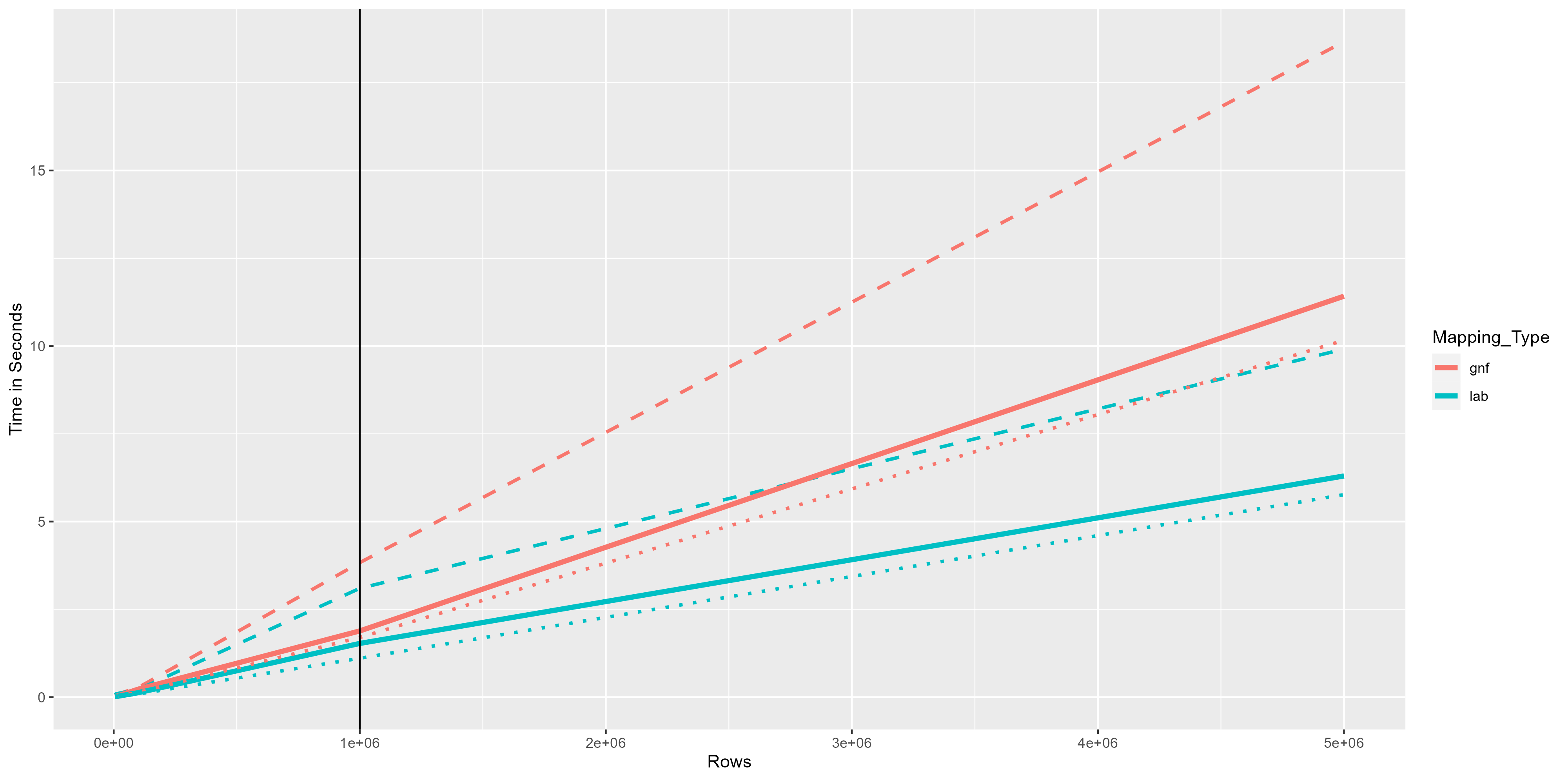
| Image 2. Results of the comparisons using Monte Carlo Simulations. |
| Strong lines represent the median, long and short dotted lines the maximum and minimum values, respectively. |
To test the time efficiency of each function I iterated each of them a thousand times using datasets of different sizes, going from 1 thousand to 5 million, measuring the time at the beginning and end of the mapping process, and extracting the difference. The graphics presented here are the Minimum, Maximum and Median values of the thousand repetitions per each function. You can see the amount of rows in the data frame plotted against the time that each function took, in seconds.
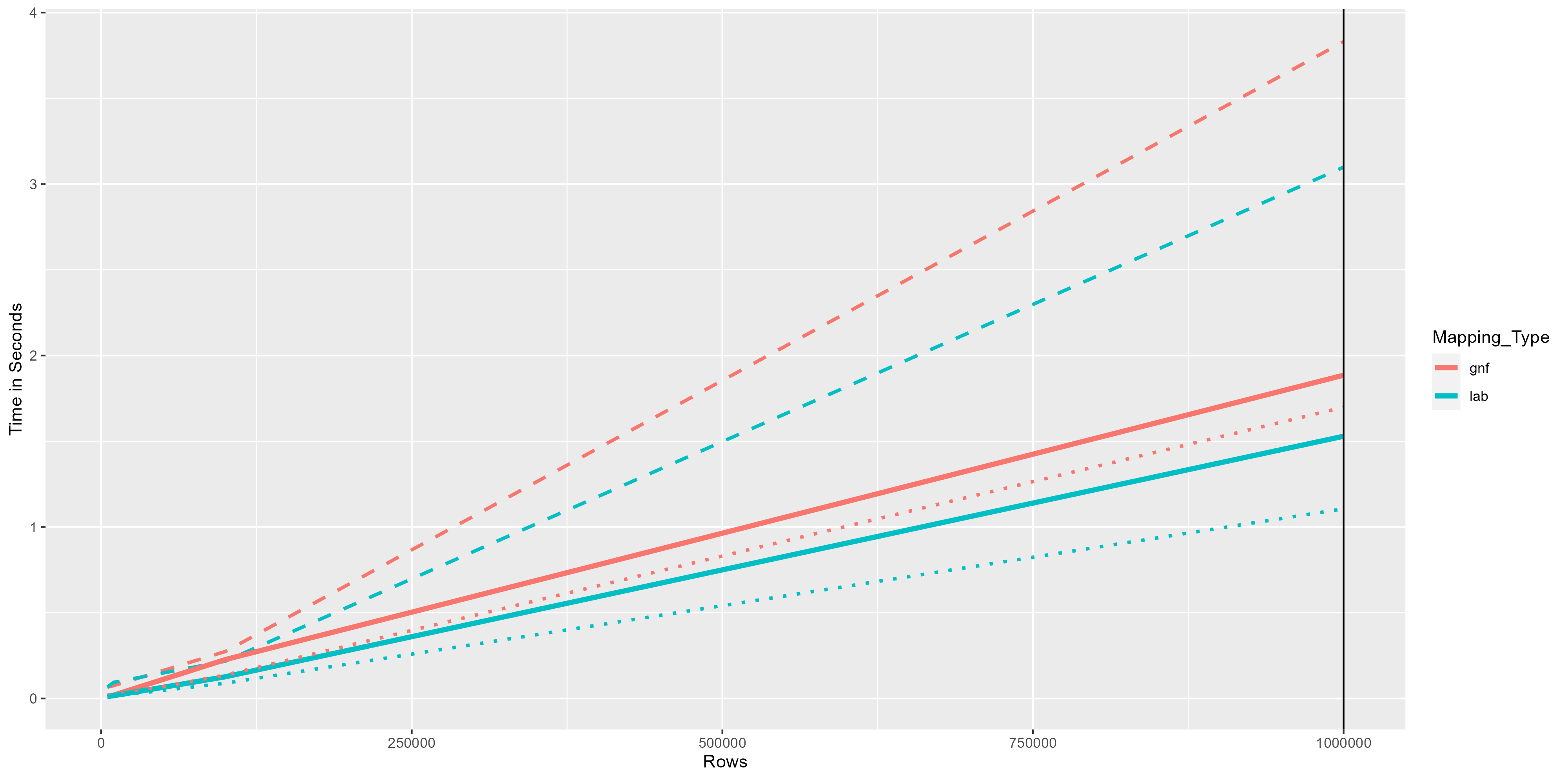
The results, as expected, show a direct correlation between time and amount of rows processed. What is interesting is that up to one million rows, the increase is very slow and the difference between methods is almost not noticeable. In the image 3 we can see that differences are smaller than 1 second. However, as the amount of rows increases above a million, the differences between methods are bigger, to a point where they even double the time.
| Image 3. Results of the comparisons up to a million rows |
| Strong lines represent the median, long and short dotted lines the maximum and minimum values, respectively. |
Conclusions
We are not using datasets above 5 million rows in the project, and even rarely above a million so, we can afford the process to take up to 12 seconds from time to time. However, there was a nice lesson to learn, especially for me: my method using base r functions is twice as slow than a method using tidyverse group of functions. That shows the commitment of R studio of making not only more human-readable functions, but also more efficient.
This is also true for a series of new packages appearing in the last years that are helping R to cope better with big data. As I mentioned at the beginning of my post, I consider myself lucky to see how R is evolving and adapting to the challenges of our times when we have the needs to process big amounts of data relatively fast. Rather than see its slow time processing as its future doom, I see it as the potential where developers are focusing to create packages that can make our job easier and be up to the challenge. And for that, I thank them!.


