This post is part of the series maps-app.
You can also find the current state of the project under my GitHub repo mapic.
Scope of this post
This is the second part of the series to create a map of any region of the world with R.
We are creating maps of data showing changes over a span of time for different countries and pointing at all kinds of cities. That basically means that we need to map any region of the world with R. Today there are all kinds of packages and techniques to do that. I will share the strategy I used with ggplot2 and maps packages, using support of Open Street Map to obtain the coordinates of cities and finally making it interactive with shiny.
This series of posts share my path towards the creation of the Shiny app. It is a live project and I decided to share my path and experiences along the creation process. The posts are not only about the Shiny app, but the package I created behind it, including topics of functions crafting, creation of the maps, classes of objects, etc., as well as any interesting issue that appear on the way. It is my way to contribute to the R community and at the same time keeping the project documented for myself.
This post is about Web scrapping with nominatim open street maps
I hope you all enjoy it. Feel free to leave any kind of comment and/or question at the end.
Open Street Maps and Nominatim
A simple query
 library('RJSONIO')

 site <- ("http://nominatim.openstreetmap.org/search?city=Texcoco&limit=9&format=json")
 (result <- fromJSON(site))
 > [[1]]
 > [[1]]$place_id
 > [1] 1177116
 >
 > [[1]]$licence
 > [1] "Data © OpenStreetMap contributors, ODbL 1.0. https://osm.org/copyright"
 >
 > [[1]]$osm_type
 > [1] "node"
 >
 > [[1]]$osm_id
 > [1] 336169214
 >
 > [[1]]$boundingbox
 > [1] "29.619"       "29.659"       "-111.0786667" "-111.0386667"
 >
 > [[1]]$lat
 > [1] "29.639"
 >
 > [[1]]$lon
 > [1] "-111.0586667"
 >
 > [[1]]$display_name
 > [1] "Texcoco, Carbó, Sonora, México"
 >
 > [[1]]$class
 > [1] "place"
 >
 > [[1]]$type
 > [1] "village"
 >
 > [[1]]$importance
 > [1] 0.385
 >
 > [[1]]$icon
 > [1] "https://nominatim.openstreetmap.org/ui/mapicons/poi_place_village.p.20.png"
 >
 >
 > [[2]]
 > [[2]]$place_id
 > [1] 3448536
 >
 > [[2]]$licence
 > [1] "Data © OpenStreetMap contributors, ODbL 1.0. https://osm.org/copyright"
 >
 > [[2]]$osm_type
 > [1] "node"
 >
 > [[2]]$osm_id
 > [1] 458633446
 >
 > [[2]]$boundingbox
 > [1] "16.551667"  "16.591667"  "-97.053333" "-97.013333"
 >
 > [[2]]$lat
 > [1] "16.571667"
 >
 > [[2]]$lon
 > [1] "-97.033333"
 >
 > [[2]]$display_name
 > [1] "Texcoco, Santa María Sola, Oaxaca, México"
 >
 > [[2]]$class
 > [1] "place"
 >
 > [[2]]$type
 > [1] "hamlet"
 >
 > [[2]]$importance
 > [1] 0.36
 >
 > [[2]]$icon
 > [1] "https://nominatim.openstreetmap.org/ui/mapicons/poi_place_village.p.20.png"
We start with Open Street Map and its API nominatim. In the piece of code above we can see how to perform a simple query for one city. It is basically one long string containing first the url of nominatim and at the end the search details: here we start the search with city using ?city=Texcoco, in this case I aimed for a city with only a few results. Next we are limiting the amount of results to 9 with &limit=9 and finally requesting the results in format JSON.
We could basically copy the string that we are passing to site and paste it in the web browser to see the results directly there. Feel free to change the city Texcoco to any other city, and play a bit more with the rest of the parameters. Particularly have a look at what happens when you remove the &format=json part or when you exchange json for any other abstract string like csv or other non-recognized format.
A more specific query
city <- 'San%20Francisco'
state <- '&state=California'
country <- '&countrycodes=US'
start.nominatim <- "http://nominatim.openstreetmap.org/search?city="
end.nominatim <- "&format=json"

site <- paste0(start.nominatim, city, country, state, end.nominatim)
(result <- fromJSON(site))
> [[1]]
> [[1]]$place_id
> [1] 297054975
>
> [[1]]$licence
> [1] "Data © OpenStreetMap contributors, ODbL 1.0. https://osm.org/copyright"
>
> [[1]]$osm_type
> [1] "relation"
>
> [[1]]$osm_id
> [1] 111968
>
> [[1]]$boundingbox
> [1] "37.6403143"  "37.929811"   "-123.173825" "-122.281479"
>
> [[1]]$lat
> [1] "37.7790262"
>
> [[1]]$lon
> [1] "-122.419906"
>
> [[1]]$display_name
> [1] "San Francisco, CAL Fire Northern Region, California, United States"
>
> [[1]]$class
> [1] "boundary"
>
> [[1]]$type
> [1] "administrative"
>
> [[1]]$importance
> [1] 1.035131
>
> [[1]]$icon
> [1] "https://nominatim.openstreetmap.org/ui/mapicons/poi_boundary_administrative.p.20.png"
If you explore OSM and nominatim a bit you will see that we can add search arguments using & followed by the argument we want (i.e., state), the symbol equal = and the argument. In my example above you can see how we are specifying the State and Country of our query. Additionally it is important to know how to pass spaces in a name, for example, San Francisco will be passed as San%20Francisco.
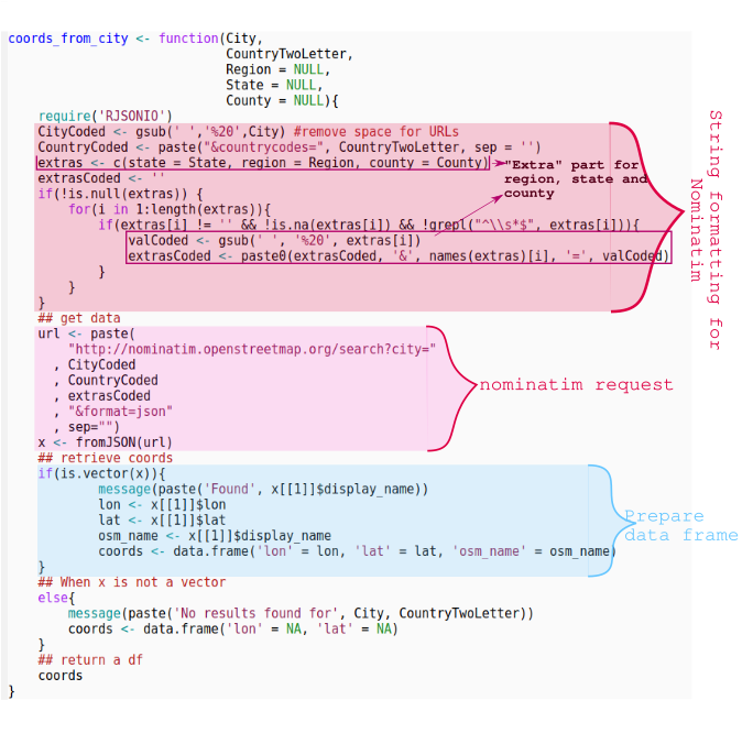
With this basic information in mind and knowing that the package RJSONIO helps us to retrieve the data from the JSON api into an R-friendly format, we can easily prepare a function to search for any city quickly, provided a few extra details like a region, state or county, and especially important, the country (try searching for cities like London or Prague without providing a country, you might be surprised of how many cities exist in the world with such names).
coords_from_city <- function(City,
                             CountryTwoLetter,
                             Region = NULL,
                             State = NULL,
                             County = NULL){
    require('RJSONIO')
    CityCoded <- gsub(' ','%20',City) #remove space for URLs
    CountryCoded <- paste("&countrycodes=", CountryTwoLetter, sep = '')
    extras <- c(state = State, region = Region, county = County)
    extrasCoded <- ''
    if(!is.null(extras)) {
        for(i in 1:length(extras)){
            if(extras[i] != '' && !is.na(extras[i]) && !grepl("^\\s*$", extras[i])){
                valCoded <- gsub(' ', '%20', extras[i])
                extrasCoded <- paste0(extrasCoded, '&', names(extras)[i], '=', valCoded)
            }
        }
    }
    ## get data
    url <- paste(
        "http://nominatim.openstreetmap.org/search?city="
      , CityCoded
      , CountryCoded
      , extrasCoded
      , "&format=json"
      , sep="")
    x <- fromJSON(url)
    ## retrieve coords
    if(is.vector(x)){
            message(paste('Found', x[[1]]$display_name))
            lon <- x[[1]]$lon
            lat <- x[[1]]$lat
            osm_name <- x[[1]]$display_name
            coords <- data.frame('lon' = lon, 'lat' = lat, 'osm_name' = osm_name)
    }
    ## When x is not a vector
    else{
        message(paste('No results found for', City, CountryTwoLetter))
        coords <- data.frame('lon' = NA, 'lat' = NA)
    }
    ## return a df
    coords
}
An important detail to know is that often, providing values to either state or region parameters returns similar results, this is particularly useful in countries where no states are used or other forms of organization are present. However, when the country has "States", you cannot pass the name of a State to the parameter Region.
The function returns a data frame that we will use later to create a table with all of our results. Since we are interested in creating maps, we only need the coordinates expressed in latitude and longitude parameters. In case the query is not found, it fills the values with NA's, which later we'll use to keep track of what was found and what wasn't. We are also keeping the values inside osm_name which provides enough information to tell the user useful details regarding the search results, including the country of the city found, and other details like state or region.
An important point to consider in coords_from_city is that it will return only the top result from the query. It means that the more information you provide, the more accurate your result will be. For our project it worked well because for big countries we were always collecting enough info about regions and states, while for smaller countries often the options were too small. But if you use the function it is important to know that if you provide a city name like Springfield, Country = 'US' and give no info about State and County, the function will retrieve only the top result from the search and discard the remaining options.
Keeping the info in a database
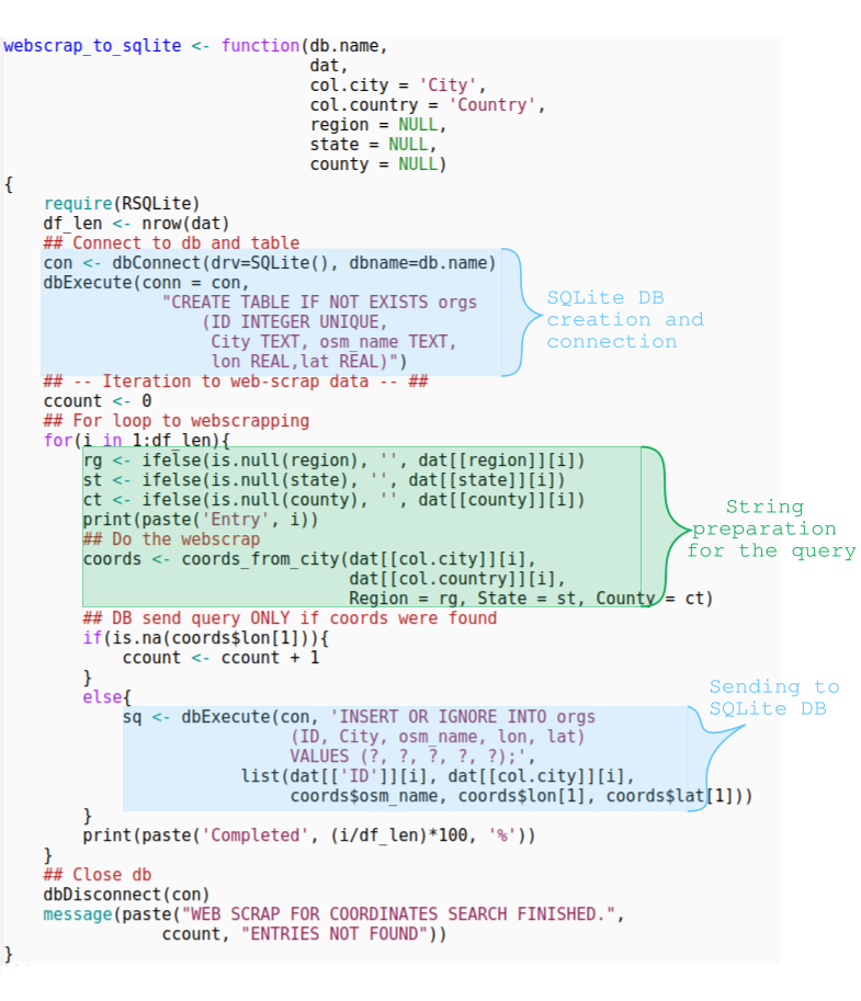
The function coords_from_city could be enough if we need to retrieve info about a few cities; we could make a for loop, retrieve all the coords we need and sore them in a data frame to later save as csv, Rdata or any format we choose. The same is true when we are searching for hundreds or thousands of cities but with data increasing the searching time also increases. If, for any reason, the R session breaks, the information would be lost and we will have to start all over again from row 1. Therefore, we are going to send every single result to a database. In that way, no matter when we stop the process or how this happens, the data is safely stored outside of R.
webscrap_to_sqlite <- function(db.name,
                               dat,
                               col.city = 'City',
                               col.country = 'Country',
                               region = NULL,
                               state = NULL,
                               county = NULL)
{
    require(RSQLite)
    df_len <- nrow(dat)
    ## Connect to db and table
    con <- dbConnect(drv=SQLite(), dbname=db.name)
    dbExecute(conn = con,
                "CREATE TABLE IF NOT EXISTS orgs
                    (ID INTEGER UNIQUE,
                     City TEXT, osm_name TEXT,
                     lon REAL,lat REAL)")
    ## -- Iteration to web-scrap data -- ##
    ccount <- 0
    ## For loop to webscrapping
    for(i in 1:df_len){
        rg <- ifelse(is.null(region), '', dat[[region]][i])
        st <- ifelse(is.null(state), '', dat[[state]][i])
        ct <- ifelse(is.null(county), '', dat[[county]][i])
        print(paste('Entry', i))
        ## Do the webscrap
        coords <- coords_from_city(dat[[col.city]][i],
                                   dat[[col.country]][i],
                                   Region = rg, State = st, County = ct)
        ## DB send query ONLY if coords were found
        if(is.na(coords$lon[1])){
            ccount <- ccount + 1
        }
        else{
            sq <- dbExecute(con, 'INSERT OR IGNORE INTO orgs
                             (ID, City, osm_name, lon, lat)
                             VALUES (?, ?, ?, ?, ?);',
                        list(dat[['ID']][i], dat[[col.city]][i],
                             coords$osm_name, coords$lon[1], coords$lat[1]))
        }
        print(paste('Completed', (i/df_len)*100, '%'))
    }
    ## Close db
    dbDisconnect(con)
    message(paste("WEB SCRAP FOR COORDINATES SEARCH FINISHED.",
                ccount, "ENTRIES NOT FOUND"))
}
For storing the data I have chosen to use SQLite through the R package RSQLite. If you are not familiar with SQL databases I recommend you to start with a general google search and then come back to the documentation of SQLite and the R package. I chose SQLite because we needed to have something light and portable that would allow us to move the information easily from country to country rather than a centralized database where we could store everything, but a very similar approach can be applied using other types of SQL databases.
The function dbConnect() generates the SQLite file if it does not exist yet. Then we give SQLite the order to create the table orgs if doesn't exist yet, and the structure for such table. Next we search for the coordinates of the entries one by one using coords_from_city() and finally we send it to the database. In that way we could stop the process at any time and continue later by simply retrieving the table orgs from the database, compare it with our original data and move forward from what is missing. For that, the column ID is critical, it is the column that allows us to link an entry between the original data, the R data.frame and the SQL table.
Our function also has a variable ccount that counts each time an entry was not found. In that way, once the query is finished it will print the amount of entries that were not found. The reasons for not finding an entry can be many, among the most common ones that I encountered are the following:
- Wrong spelling of the City name or excess of info (i.e., value "Prague, District 3" when the city name is simply "Prague").
- Wrong spelling of the State, Region and/or County name.
- The given City is simply not in the database of Open Street Maps (it happened specially for very small villages).
- Breaks of the internet connection. This one is particularly important because sometimes running the query a second or third time would find cities that were not found the first time.
To read the data back to R from SQL we simply need to make a connection to the database, read the table, and close the connection. The function combine_df_sql takes care of that and at the same time joins our original data to the data stored in the database by the ID and the city name. This was important for the project because we wanted to keep the coordinates of the cities separated from the rest of the information due to some internal practical reasons. But I think that keeping all the data in SQL at once can facilitate many things. Among others, you could identify when a particular city was already found in the past and retrieve the coordinates from the database directly rather than making a connection to nominatim. I did that for a few countries and it reduces the querying time considerably. For the present post I decided to show the separated version of data in order to provide more tools to the reader.
combine_df_sql <- function(db.file, original.data){
    require(dplyr)
    require(RSQLite)
    if(is.character(original.data)){
        if(grepl('.csv', original.data, fixed = T)){
            df <- read.csv(original.data)
        }
        else{
            stop("Incorrect file format for data")
        }
    }
    else if(is.data.frame(original.data)){
        df <- original.data
    }
    else{
        stop("Incorrect data format")
    }
    con <- dbConnect(drv=RSQLite::SQLite(), dbname = db.file)
    db <- dbReadTable(con, "orgs")
    dbDisconnect(con)
    result <- left_join(df, db, by = c('ID', 'City'))
    return(result)
}
Another detail of our function is the ability to read either from the csv file or from a data.frame. Since we were working mainly with csv files and I used data frames for the unit tests, these 2 formats were enough. Feel free to modify or extend the function for the data formats that you might need.
Missing data
As mentioned above, sometimes the results from the query would be incomplete and a second or third run were necessary but with a fewer rows. Some others I just needed to stop the query and continue later from where we left. And yet some other times the data was incomplete or wrong and this could be solved later with the data owner. The 3 scenarios required me to read the csv file to R, then the table from the database and compare them to filter the missing values. So I crafted the function compare_db_data to compare the database (db) to the original data.
compare_db_data <- function(db.file, dat){
    require(dplyr)
    require(RSQLite)
    if(is.character(dat)){
        if(grepl('.csv', dat, fixed = T)){
            df <- read.csv(dat)
        }
        else{
            stop("Incorrect file format for data")
        }
    }
    else if(is.data.frame(dat)){
        df <- dat
    }
    else{
        stop("Incorrect data format")
    }
    con <- dbConnect(drv=RSQLite::SQLite(), dbname = db.file)
    db <- dbReadTable(con, "orgs")
    dbDisconnect(con)
    filtered <- filter(df, !(as.character(ID) %in%
                              as.character(db$ID)))
    filtered
}
As mentioned earlier, sometimes Open Street Maps would simply not have registered certain "cities" (in fact it happened only with really small villages or populations). For that the function add_coords_manually would take a csv file with a particular structure to add the missing data. The csv file must have the following columns:
IDcolumn named exactly like that and containing the same ID as the original data.- A column containing the name of the city
- Columns containing the Latitude and Longitude were we want to point at the city
- A value for
osm_name. This could be left empty or we can provide the value we want in this slot. What is important is to have the column present in the csv file.
Then, as in previous function, we pass to add_coords_manually the name of the csv file with the complementary information, the name of the SQLite database and the names of the columns where we have the values for city names, osm_name, lat and long, all as strings. The rest of the function is self descriptive, provided basic knowledge of SQL syntax.
add_coords_manually <- function(csv_file, db.name,
                                city, osm_name, lat, lon){
    require(tidyverse)
    require(RSQLite)
    csv_dat <- read_csv(csv_file)
    csv_len <- length(csv_dat$ID)
    con <- dbConnect(drv=RSQLite::SQLite(), dbname=db.name)
    for(i in 1:csv_len){
        dbSendQuery(con, 'INSERT OR IGNORE INTO orgs
                      (ID, City, osm_name, lon, lat)
                      VALUES (?, ?, ?, ?, ?);',
                    list(csv_dat[['ID']][i],
                         csv_dat[[city]][i],
                         csv_dat[[osm_name]][i],
                         csv_dat[[lat]][i],
                         csv_dat[[lon]][i]))
    }
    dbDisconnect(con)
    print(paste(csv_len, 'inserted'))
}
Next steps
If you are new to R you could probably already had noticed that one of the strengths of R that I'm using a lot here is its use of functions. The first maps that we created were done writing scripts with a few hundreds of lines. Those gave us the basis to craft the necessary functions and so, the rest of the maps were possible using just a few lines. Some of the scripts for the web scrapping of the coordinates consist of less than 10 lines of code. That is possible using the functions above and a few others created for special or particular cases. I will not share absolutely everything but I want to give an idea of how to make the process more efficient. You can always create more functions for your particular cases or modify my proposed functions to adapt to your particular situation.
And speaking of extensibility, just while writting this blog I found out about the package tmaptools which contains the function geocode_OSM which uses nominatim to retrieve the coordinates of the searched point. The function has a more user friendly searching format and more possibilities for the return value, while my coords_from_city() option stays quite stiff and still with the original format that it was envisioned a few years ago when I created it. If you are truly interested in the topic I invite you to check the package. Myself I have been busy maintaining the code and creating maps that I found little time to do any improvements to the original project. But that's exactly my main task right now so, if I do any changes to the functions presented here using the tmaptools package you can be sure that I will create a short post to share it as well.
Then, once we got the coordinates of our target cities and we know how to make the basic map, the next step is to add the cities to the base map. In the next post I will show you how I did that and a function to make the process faster and efficient.


